Final Report

Introduction/Background

With the rate of respiratory ailments on the rise, the stress imposed on global health becomes more prevalent [1]. These ailments, if left untreated, can leave an individual with irreversible damage to their respiratory system by impairing lung function. Recent developments in medical technology have yielded datasets of recorded lung sounds, opening up new possibilities for automated lung sound examination.

We analyze the largest and most prominent of these datasets, ICBHI [4, 5]; this dataset consists of 920 annotated recordings (via 4 different devices) from 126 patients totaling 5.5 hours and 6898 breathing cycles, as well as structured data on each patient’s age, sex, height, weight, and respiratory disease.

Problem Definition

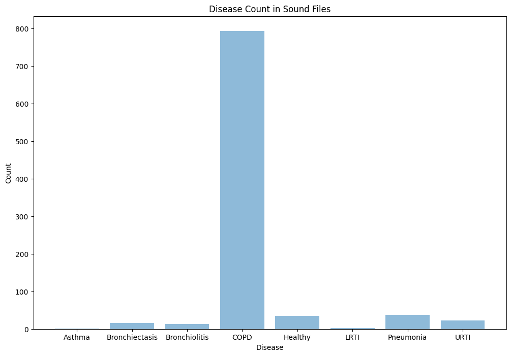
Motivated by our desire to improve early detection of serious respiratory disease, we analyze audio samples using machine learning methods to differentiate between 6 different kinds of respiratory conditions (COPD, URTI, Bronchiectasis, Pneumonia, Bronchiolitis, and healthy) as a way of pre-screening patients. We believe this project will be best utilized as a web application to expedite triage in medical establishments or to enhance at-home symptom checking. While most published work on the topic has focused on identifying abnormal sounds, such as crackles and wheezes, with high levels of accuracy [1,2,6], we go further and attempt to identify the specific pulmonary disease of a patient given their demographic information and auscultation audio sample.

Methods and Results (Will be discussed together for each model)

Preprocessing

Our dataset consists of various audio files in .wav format. Each audio file contains several breathing cycles that may have crackles and/or wheezes. The timestamps for the breathing cycles, as well as whether a crackle or wheeze was detected, are found in the .txt file that corresponds to a given .wav file. The initial phase of our preprocessing involves splitting all the 920 .wav files into separate audio clips given by the timestamps in the corresponding .txt files. We store the 6898 newly preprocessed audio files in a folder called clips_by_cycle. Next, we generate mel spectrograms from these clips. These spectrograms visualize each audio clip in the following manner: the x-axis represents the timestamp of a given sample within the cycle, the y-axis represents a certain frequency bucket, and the intensity of the color of each time-frequency square associated with the spectrograms represents the magnitude of the given frequency at that time. Then, we join the demographic data from demographic_info.txt with our mel spectrogram .jpg files and our .wav clips by cycle on patient ID and cycle number. Additionally, we add a BMI column as we have some child heights and weights. Our final data frame includes patient id, cycle number, start and end timestamps, whether a crackle and/or wheeze was detected in each cycle, chest location and acquisition position, recording equipment, the audio clip for the cycle, the mel spectrogram for the cycle, and BMI, amongst other columns. For future use, we implement an additional step in our preprocessing that can be used for the supervised learning models. We first downsample the files to 4KHz, as the sampling rate is different for each file. Then we use a 5th order butter band-pass filter that removes background noise such as background speech, and heartbeat. We then standardize and normalize the audio clips. These three preprocessing steps are complete on each audio file and add to another folder for future utilization. We then generate spectrograms using these preprocessed audio clips and save these in a folder called normalized_spectrograms. In addition to using these normalized spectrograms and preprocessed audio clips for the supervised learning models, we will compare our findings from the unsupervised GMM model from the old spectrograms and the newly preprocessed ones.

GMM

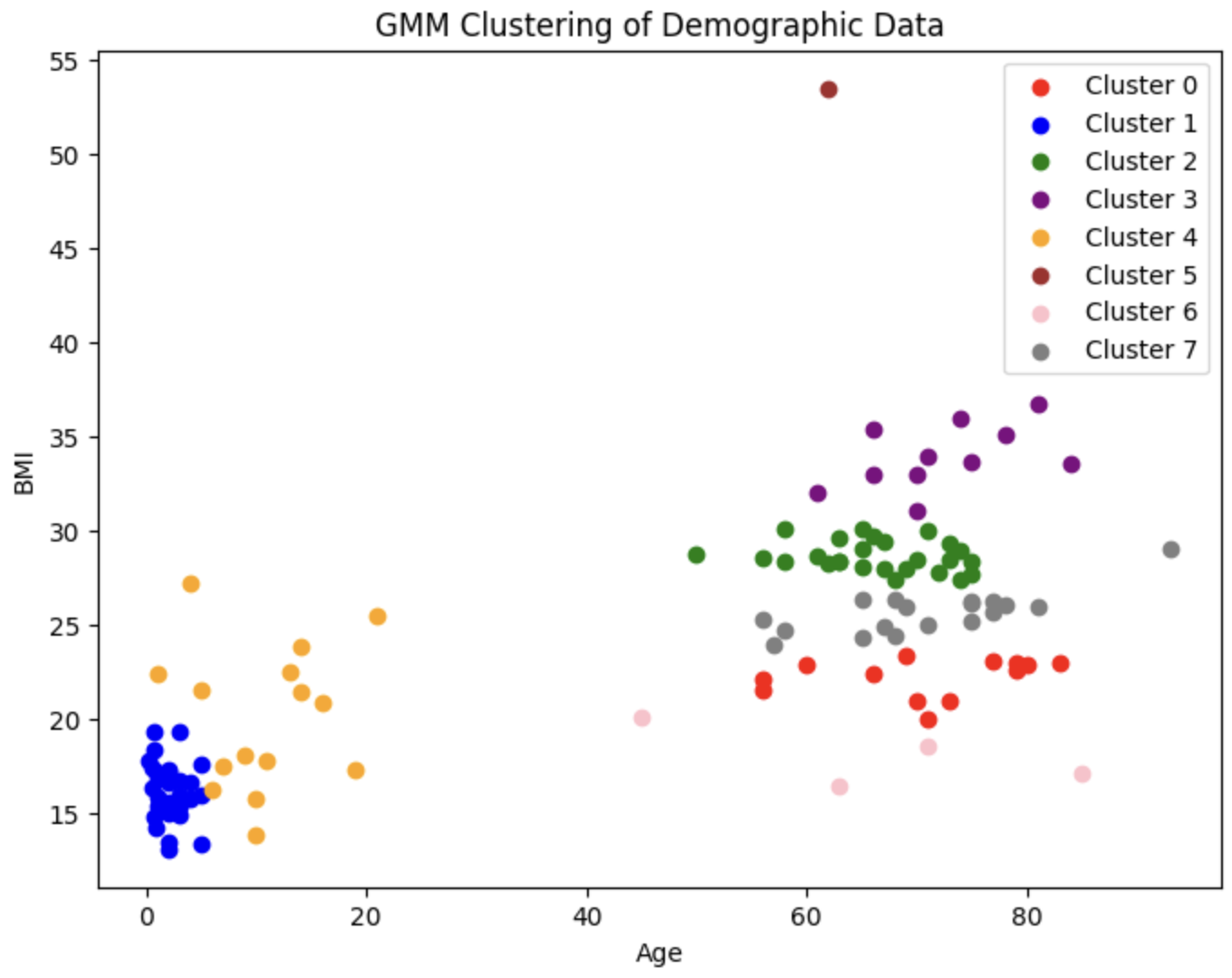
Before we approach the problem of analyzing the audio samples with supervised learning methods, we wish to visualize the distribution of the patients and observe whether there exist any clusters of patients that are predisposed to each of the 8 diseases (7 diseases and healthy) we will be classifying between. We first fit a Gaussian Mixture Model (GMM) on the most relevant demographic features present in the demographic data (namely age and bmi). We choose to use a GMM over other unsupervised learning methods, as GMM is a soft-clustering method; it returns responsibility probabilities that can give us a general idea of how likely a given datapoint (i.e. patient) is to be in each of the 8 clusters (i.e. have each of the 8 conditions), which could prove to be useful for diagnosis.

Since there are 7 diseases and 1 healthy category, we choose to create 8 clusters. This is the resulting plot:

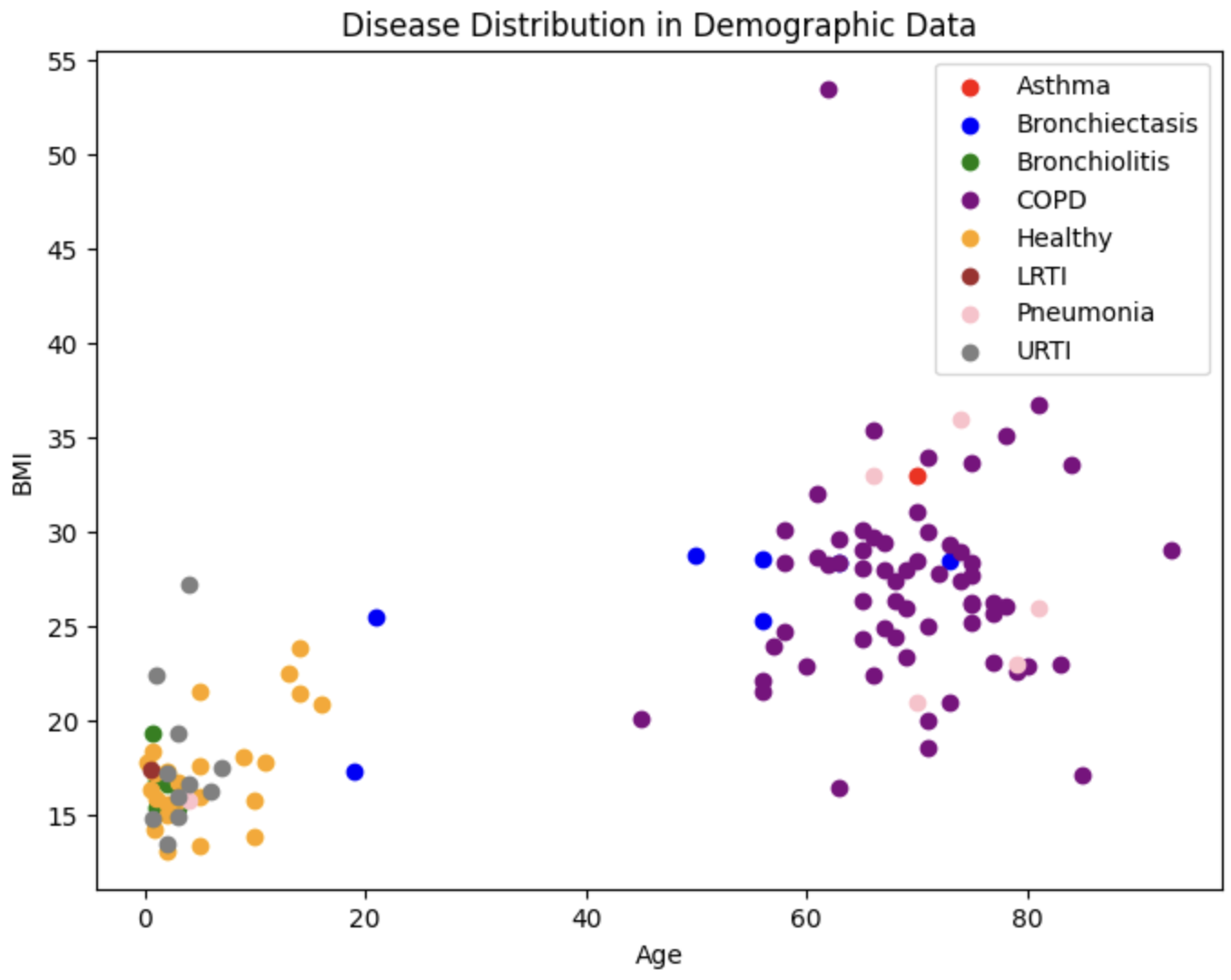We also plot the true diseases for each of these patients

To evaluate the performance of our GMM, we use both an internal measure, silhouette coefficient, and an external measure, completeness score. The silhouette coefficient is intended to measure how well-defined the found clusters are. Our clustering obtained a silhouette coefficient of .376, which is less than the desired threshold of at least 0.5, indicating that the GMM did not return tight clusters that are spread out (i.e. our clusters are not well-defined). The completeness score is intended to measure how well the clusters of our GMM align with the true distribution of the patient diagnoses. Using the diseases as the true labels, we obtain a completeness score of .388. As completeness scores near 1 reflect better clusterings of our data with respect to the true diagnoses, this once again is a poor result. These metrics and the corresponding visualizations suggest that GMM clustering does not provide as much information about more susceptible populations as we would have hoped. However, one interesting observation to note is that patients who have one of LRTI, Bronchiolitis, URTI (or are healthy) tend to lie in a very different area of Age-BMI space than patients with COPD, Asthma, and (oftentimes) pneumonia. Hence, for our next steps, we will experiment with training a GMM on just these two macro-classes of diagnoses to try to extract insights that may be useful in our supervised analysis.

PCA

These mel spectrograms are 200x500 images; hence, each spectrogram is composed of 100,000 features. In order to greatly reduce the number of features and decrease our future models’ (both the unsupervised and supervised models to be applied on the audio files) complexity, we apply principal component analysis (PCA) on spectrograms. We use PCA on a sample of 1000 spectrograms in order to get an estimate for how many components are needed to retain at least 99% of the original variance. We choose a relatively large cutoff of 99%, as spectrograms contain high-fidelity data that must be kept intact. Below, we visualize the total explained variance ratio as a function of the number of kept principal components (image right-trimmed for brevity).

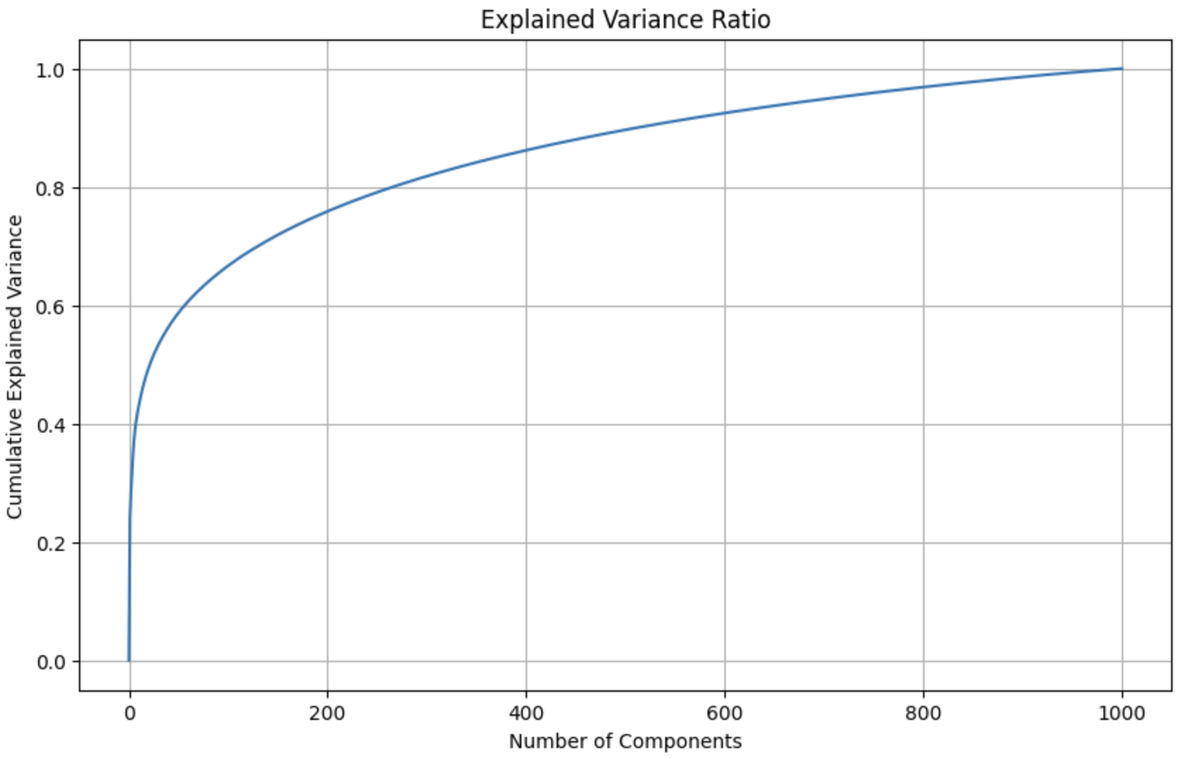Number of components required to explain 99% of the variance: 927

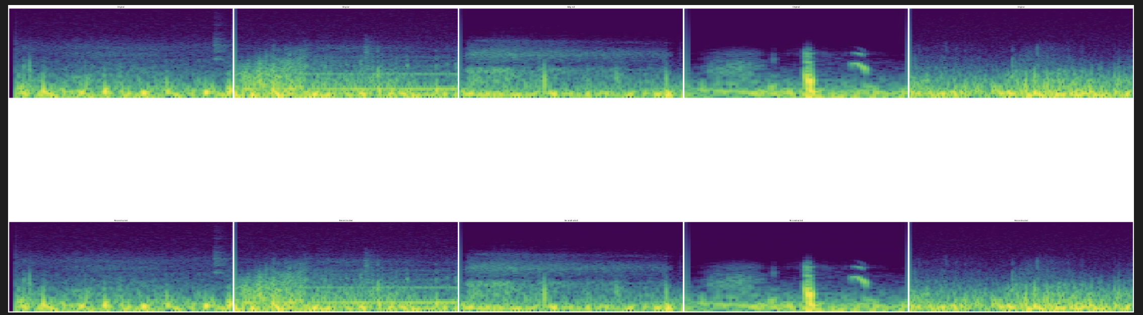We visualize 5 examples of spectrograms. The top row depicts the 5 original spectrograms (100,000 features), and the bottom row depicts the reconstruction of these spectrograms from the top 927 principal components.

Audio Clustering

A more interesting unsupervised task is the analysis of the audio files themselves. We look to answer the question: are there any visualizable patterns in the audio files that may indicate the existence of certain diseases? We take inspiration from [8] for the following analysis.

To do this, we first begin by extracting Mel-frequency cepstrum coefficients (MFCCs) from each preprocessed audio clip. MFCCs are a common method of summarizing audio, and they have been shown in [9] to be a good predictor of the disease associated with a certain ICBHI dataset audio file, making it an appropriate choice for our task.

We extract 13 MFCCs from each audio snippet. 13 MFCCs is the most widely used dimension for MFCC extraction across a variety of audio applications, as an MFCC vector of size 13 is able to capture most of the variance of an audio file; extracting more than 13 does not retain much more information, extracting fewer than 12 do not capture enough information. Furthermore, we verified this choice by performing the clustering and analysis that follows with various MFCC dimensions ranging from 10 to 20, and found that 13 consistently gave us the best results for a reasonable computational cost.

Then, we use an unsupervised dimensionality reduction technique known as t-SNE [10] (t-distributed Stochastic Neighbor Embedding) to visualize projections of the MFCCs onto a 2D plot. Note that we elect to use t-SNE over PCA in this case, as we are primarily concerned with the visual properties of our projection, and not as much the preservation of variance. t-SNE more accurately visualizes the relative similarity of datapoints, as it keeps similar datapoints close together in the 2D projection, but separates dissimilar datapoints.

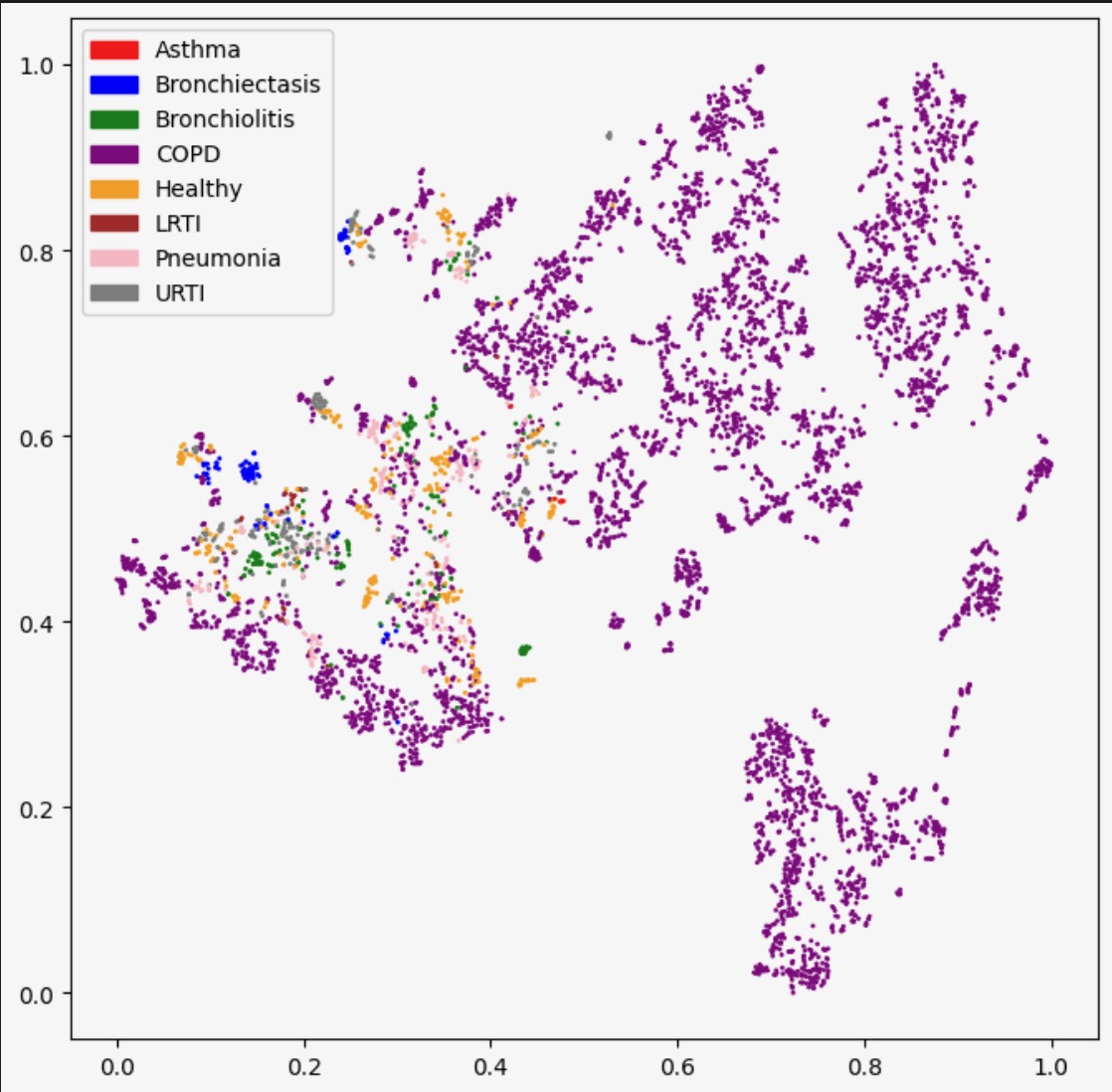
This is the resulting plot of t-SNE applied to our MFCCs with different hyperparameters (i.e. number of iterations and perplexity). Each datapoint is colored by the true disease it is associated with.

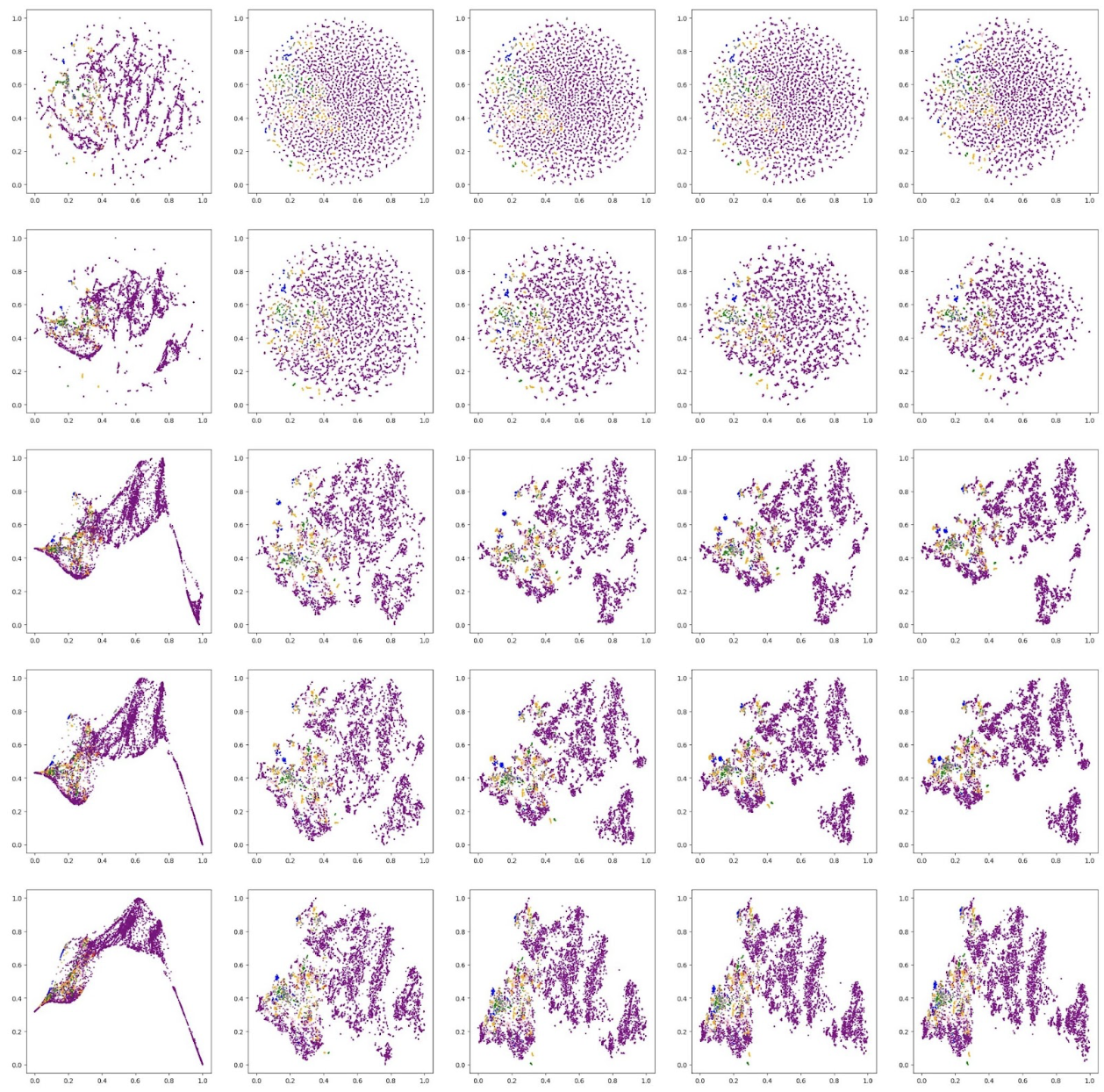
Based on these visual results, we qualitatively decide that the plot generated by perplexity of 30 and 5000 iterations is the best.

Now, we cluster these dimension-reduced datapoints using DBSCAN. We decided to use DBSCAN because the shapes of the apparent clusters in our t-SNE plot do not resemble clean circles (which would suggest k-means is the appropriate algorithm) or ellipses (GMM); rather, they resemble arbitrary dense areas. Because DBSCAN is sensitive to epsilon, and not its other parameter min_pts, we fix min_pts at 5 and test different values of epsilon for our clustering, as shown below (note: we tested many other values of epsilon, but for the sake of readability, we only present 3 examples):

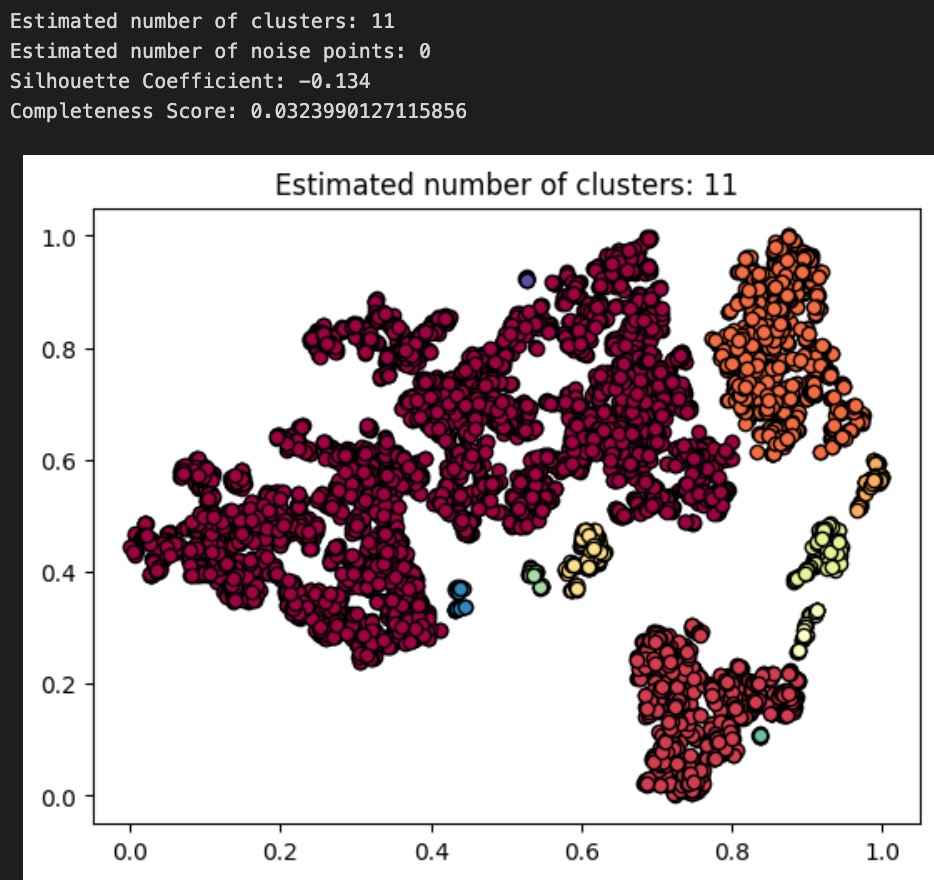
Above: plot and results for DBSCAN(min_pts=5, epsilon=.03)

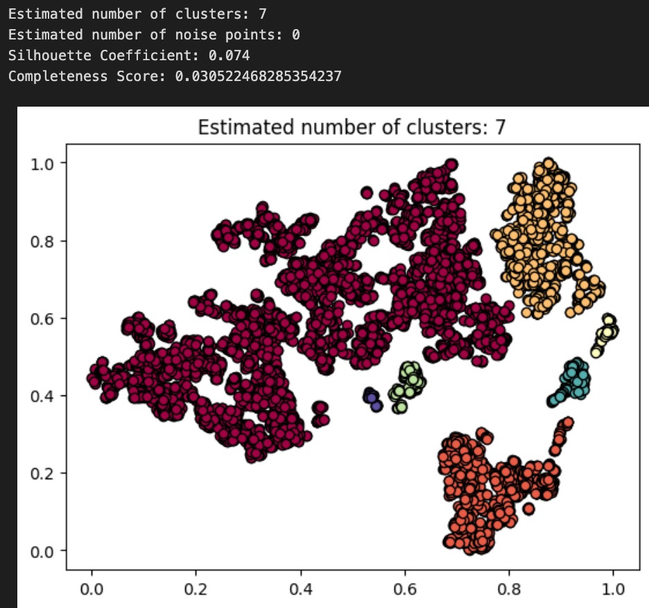
Above: plot and results for DBSCAN(min_pts=5, epsilon=.035)

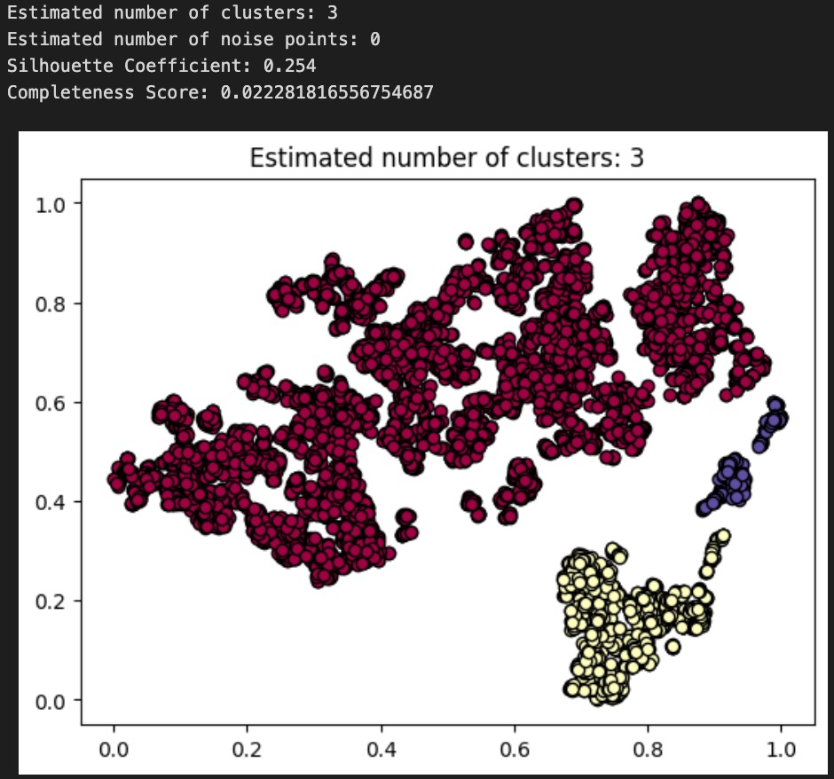
Above: plot and results for DBSCAN(min_pts=5, epsilon=.05)

To evaluate the performance of each of our DBSCAN clusterings, we use both an internal measure, silhouette coefficient, and an external measure, completeness score, just as we did to evaluate our GMM from earlier. Our clusterings obtained silhouette coefficients of -.134, .074, .254, indicating that an epsilon of .05 gives us the tightest, most well-defined clusters. All of these are less than the desired threshold of at least 0.5, indicating that none of the DBSCAN algorithms returned well-defined clusters. Using the diseases as the true labels, we obtain completeness scores of .032, .031, and .022, indicating epsilon values of .03 and .035 give roughly equal results (better than epsilon of .05) when it comes to the predictive value of our clusters. As completeness scores near 1 reflect better clusterings of our data with respect to the true diagnoses, this once again is a poor result. As a final decision, we elect to go with our epsilon=.035 clustering as our final assignment, as this clustering has the nice property of having 7 clusters, which is very close to the true number of diseases there are. These metrics and the corresponding visualizations suggest that DBSCAN clustering of the audio files alone do not provide as much information about the disease an audio file might relate to as we would have hoped. Though these results are poor, they are to be expected, as the question of determining what disease a patient has is quite a difficult problem, as evidenced by the mere existence of the ICBHI challenge and the numerous research papers published on the topic by Microsoft, MIT, and other leading research organizations.

We now compare the results of our GMM clustering with that of our DBSCAN clustering. Interestingly enough, our completeness scores were far higher (10x) when using GMM on the demographic data than for DBSCAN on the audio files. This implies that the demographic data of a patient is a far better predictor of the disease they might have, as compared to a simple audio recording. For future analysis and next steps, we propose combining the MFCCs and demographic data to see if better clusterings can be obtained there. Furthermore, it may make sense to first split the audio files up based on their chest acquisition location and recording equipment, then viewing those clusters separately.

CNN

We decide that a convolutional neural network (CNN) is an effective method to implement as we aim to predict whether an individual has a particular respiratory disease.

We preprocess our audio files using a butterworth filter and standard normalization from the midterm, and we save these downsampled clips in a separate folder. We perform some data augmentation on the dataset, including a stretch and pitch shift. Next, we extract features from the clips, including the Mel-frequency cepstral coefficients (MFCCs), sampling means, and mel spectrograms. Next, we engineer the dataset by removing the singular asthma entry.

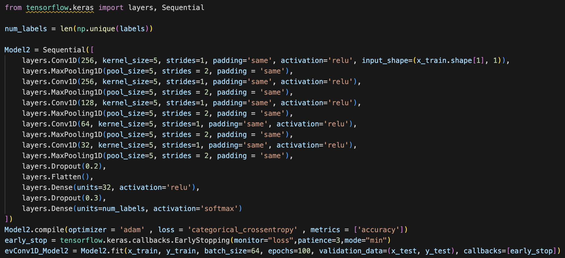
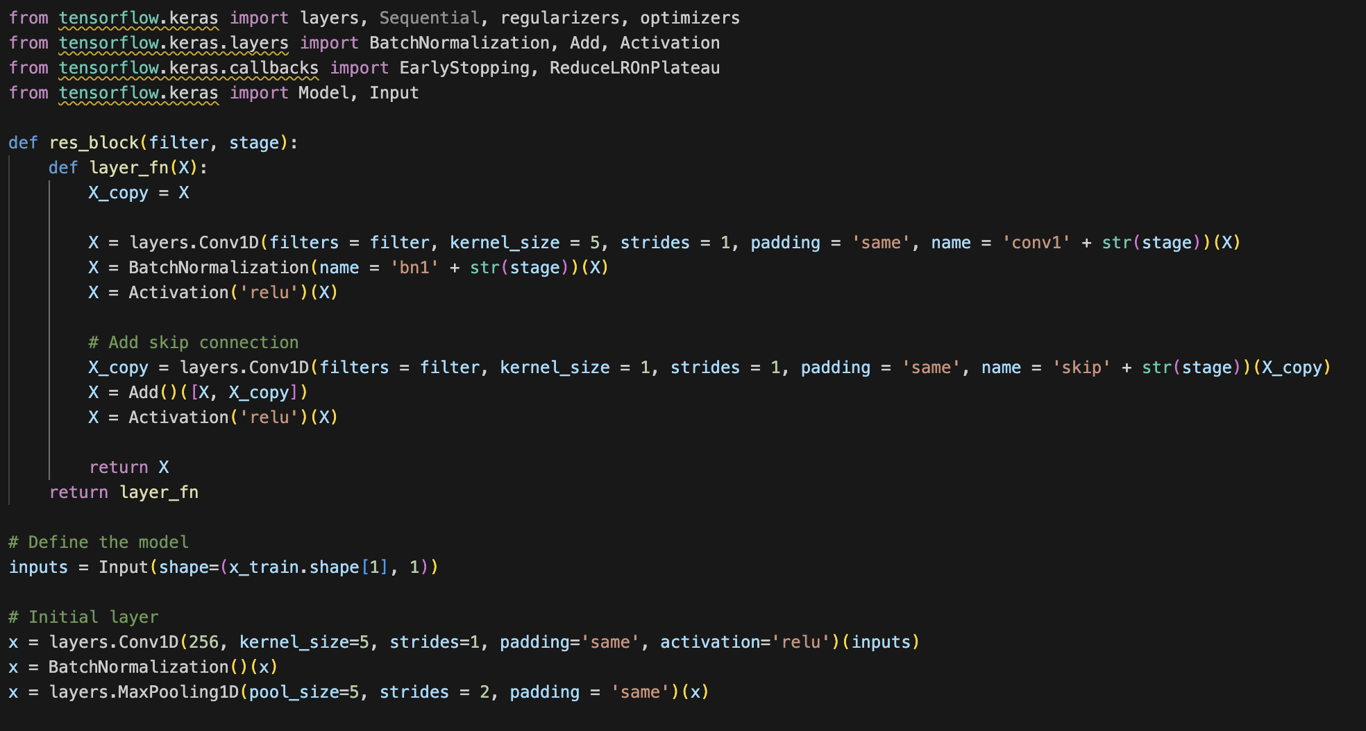
Note: Since our CNN is architected with the purpose of specifically classifying spectrograms, and not general images, we elect to use 1D convolutions instead of the standard 2D convolutions used by most image classification nets. This is because spectrograms are particularly informative in the x axis (the timestep axis). The y-axis consists of log Mel filterbank bins, and so we conclude that each row of the spectrogram is best analyzed separately. Therefore, we determine that 1D convolutions can better capture the time sequential nature of an audio file in the x axis across each one of the individual filter banks (y axis bins). The dense layers following these convolutional feature extractors take care of modeling the interaction effects between each one of the spectrogram rows.

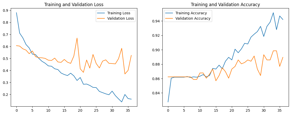
Using 1D convolutions, 1D max pooling, kernel_size of 5, and some dropout, flatten, and dense layers, our first model has a training accuracy of 0.9583 and validation accuracy of 0.8877. Our training loss was 0.1319 and validation loss of 0.5592. The code, accuracy and loss graphs, and convolution matrix for our first model is below.

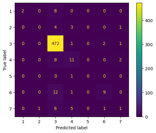
Note: the convolution matrix is labeled 1-7, which represents the following labels respectively: [Bronchiectasis, Bronchiolitis, COPD, Healthy, LRTI, Pneumonia, URTI]

We notice that the validation loss is significantly greater than the training loss, which is indicative of the model overfitting. Additionally, we aim for a validation accuracy greater than 0.9, so we make the following changes to the model: Add a residual block with skip connections to facilitate smoother gradient flow and combat the vanishing gradient problem Incorporate batch normalization to improve training stability and speed by normalizing the input of each layer Increase dropout rate to make the network more robust to variations and noise in the input data Increase regularization by adding L2 regularizers to mitigate overfitting Introduce lr_reduction to introduce a dynamic learning rate The code for the new model, accuracy and loss graphs, and convolution matrix is below.

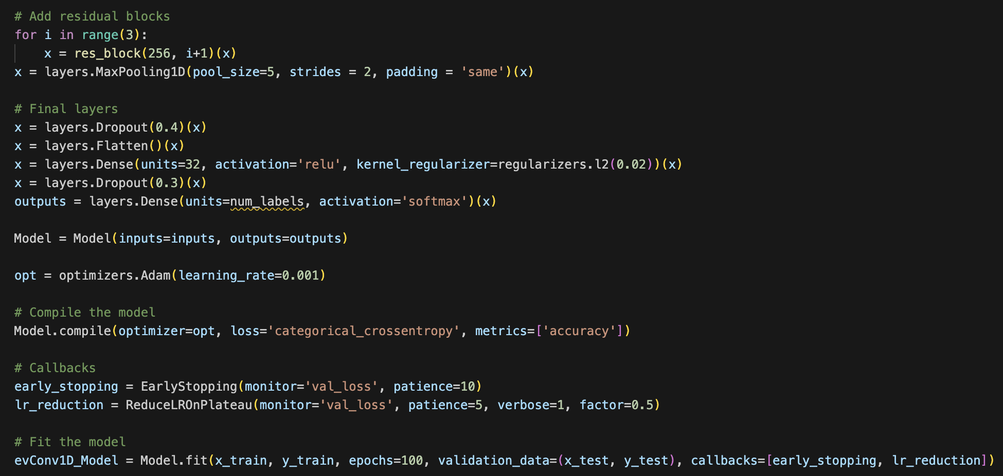
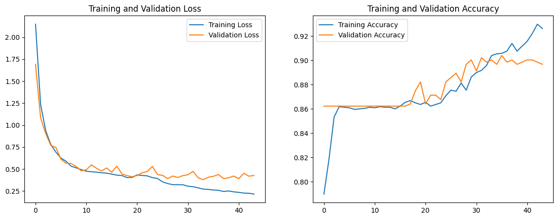
We note that the validation loss nearly mirrors the training loss until around the 20th epoch, and this also can be seen when observing the trend of training and validation accuracy. The validation accuracy was quite high at 0.906, but we aim for higher in the next model. We conclude that because the validation loss is double the training loss around the 40th epoch, the model is overfitting. To combat this issue, we increase the dropout to 0.6 for both layers. Additionally, we change the parameter for regularizers to 0.03 instead of 0.02. The accuracy/loss graphs and convolution matrix below are representative of these changes.

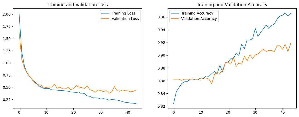
We note that the overfitting issue still persists, but the validation accuracy increased to 0.913. The training accuracy is increased to 0.962, which indicates that the model is overfitting to the training set, but the validation accuracy is high enough to justify a higher validation loss. We run one more model, in which we increase epochs to 200, reduce residual block iterations from 3 to 2, and reduce the dropout rate back to 0.4 and 0.3 respectively. The graph and convolution matrix can be found below.

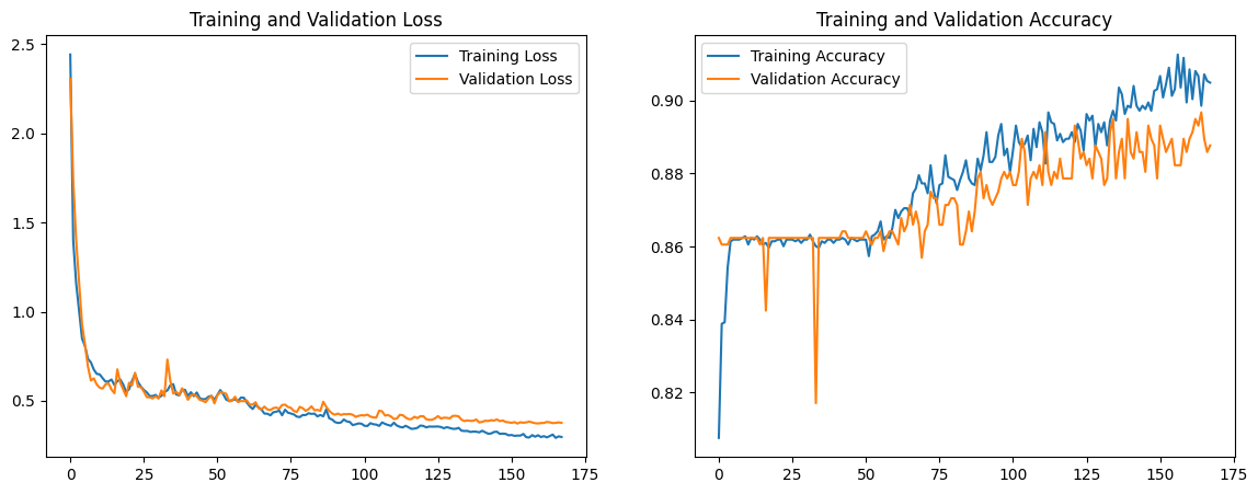
We note that the validation curve follows a similar trajectory to the training loss curve, and the validation loss decreases to 0.427. However, both the training and validation accuracy decrease by around 0.02.

The model with the best accuracy was Model 3. The features of this model that were different from other features was the increased dropout and regularizer parameter as well as the continued implementation of the residual block, block normalization, and other changes made from model 1 to model 2. Model 3 had a 2.85% improvement from the original model, and we notice that the loss and accuracy were less variable.

Next Steps

Since this project is fairly large scale, we plan on having short and long term goals. For the short term we will build a random forest (RF) to model the mix of categorical and continuous variables in our dataset. We will experiment with ensembles of these models such as feeding the input of the neural net embeddings, scores, and probabilities into the random forest. Additionally, we want to better develop our CNN architecture for the future. As for the long term, we would like to focus on developing or finding a better or more balanced dataset where we can properly run our models on this dataset as our dataset is heavily skewed COPD. Additionally, when we find or develop the new dataset we can look at other diseases that might develop in this chest area with similar tracking devices or in similar locations.

References

[1] S. Bae et al., “Patch-Mix Contrastive Learning with Audio Spectrogram Transformer on Respiratory Sound Classification,” in INTERSPEECH 2023, ISCA, Aug. 2023, pp. 5436–5440. doi: 10.21437/Interspeech.2023-1426.

[2] S. Gairola, F. Tom, N. Kwatra, and M. Jain, “RespireNet: A Deep Neural Network for Accurately Detecting Abnormal Lung Sounds in Limited Data Setting,” in 2021 43rd Annual International Conference of the IEEE Engineering in Medicine & Biology Society (EMBC), Nov. 2021, pp. 527–530. doi: 10.1109/EMBC46164.2021.9630091.

[3] Y. Cui, M. Jia, T.-Y. Lin, Y. Song, and S. Belongie, “Class-Balanced Loss Based on Effective Number of Samples,” in 2019 IEEE/CVF Conference on Computer Vision and Pattern Recognition (CVPR), Jun. 2019, pp. 9260–9269. doi: 10.1109/CVPR.2019.00949.

[4] “Respiratory Sound Database.” Accessed: Feb. 22, 2024. [Online]. Available: https://www.kaggle.com/datasets/vbookshelf/respiratory-sound-database

[5] B. M. Rocha et al., “Α Respiratory Sound Database for the Development of Automated Classification,” in Precision Medicine Powered by pHealth and Connected Health, vol. 66, N. Maglaveras, I. Chouvarda, and P. De Carvalho, Eds., Singapore: Springer Singapore, 2018, pp. 33–37. doi: 10.1007/978-981-10-7419-6_6.

[6] A. H. Sabry, O. I. Dallal Bashi, N. H. Nik Ali, and Y. Mahmood Al Kubaisi, “Lung disease recognition methods using audio-based analysis with machine learning,” Heliyon, vol. 10, no. 4, p. e26218, Feb. 2024, doi: 10.1016/j.heliyon.2024.e26218.

[7] Y. Gong, Y.-A. Chung, and J. Glass, “AST: Audio Spectrogram Transformer,” in Interspeech 2021, ISCA, Aug. 2021, pp. 571–575. doi: 10.21437/Interspeech.2021-698.

[8] L. Fedden, “Comparative Audio Analysis With Wavenet, MFCCs, UMAP, t-SNE and PCA,” Medium, Nov. 21, 2017. https://medium.com/@LeonFedden/comparative-audio-analysis-with-wavenet-mfccs-umap-t-sne-and-pca-cb8237bfce2f (accessed Apr. 24, 2024).

[9] P. Zhang, A. Swaminathan, and A. Uddin, “Pulmonary disease detection and classification in patient respiratory audio files using long short-term memory neural networks,” Frontiers in Medicine, vol. 10, Nov. 2023, doi: https://doi.org/10.3389/fmed.2023.1269784

[10] L. Com and G. Hinton, “Visualizing Data using t-SNE Laurens van der Maaten,” Journal of Machine Learning Research, vol. 9, pp. 2579–2605, 2008, Available: